Scaling and Comparing Performances of Aircraft Models (2D/3D Wing Loading) Andrej Marinsek shares his views on this topic.	The February EFO Zoom Meeting Highlights: Denny Sumner's Ace Whitman 18" Mooney Mite, rechargeable AA Lithium batteries and the Dreamer Bipe.
Pete Waters' Latest Model Pete Waters shares photos of his 1945, all aluminium, high-wing model plane.	Skymasters Indoor Flying 2021/2022 Skymasters' president, Pete Foss, fills us in on the indoor flying season in Pontiac, with some updated notes by Ken.
Indoor Flying at the Legacy Center in Brighton, MI Indoor Flying Announcement in Brighton, MI!	Upcoming E-vents
Send Ken email

Scaling and Comparing Performances of Aircraft Models (2D/3D Wing Loading) By Andrej Marinsek 1. Introduction      Many years ago (Model Airplane News, Dec. 1997) an article was published in this magazine titled "3D Wing Loadings" (Three dimensional wing loadings) by Larry Renger; it was recently published again on the internet in a slightly cleaned up version. Its different approach to a specific modeling subject is interesting but, as it will be shown later, has some problems. The concept of the 3DWL, though correct in one respect, has otherwise rather limited reach and leads to some vague interpretations and questionable conclusions. The 3DWL persists around in different forms and publications and seems to be, nowadays, the most advertised and supposedly even the only appropriate approach for estimation and comparison of some model performances. This is somehow surprising, so it needs to be addressed in some way. 2. General remarks      Coherent units from the International System of Units (SI) are used in calculations as they are clearer. In most cases only one unit is attributed to a certain physical property and numerical transformations are simpler or not needed at all.      Instead of the term weight (W), which is strictly speaking, a kind of force, the expression mass is used (designated by the letter m), which is the proper name for the physical property measured in kg (lb., oz., etc), and is employed in all calculations here. 3. Agility of models      The motion of models in the air can be on one side described by the words like "agile" or "hot" or "docile" or "flyable" or whatever expression is used to appreciate the performance of models in flight. However this can be pretty undetermined and subjective.      On the other hand, some objective (given by numbers) performance parameters exist. With regard to the lateral axis of models, some performances directly depend on the lift force. These are the minimal speed in horizontal flight vm (stall speed), the minimal absolute turning (or circling) radius Rm and the minimal relative turning radius (RTm), which will be defined and discussed a bit later.      Also, some settings (such as the center of gravity) and a number of model properties, for instance wing profile, low/high wing, aspect ratio, tail (distance from the wing, area, position), the size of rudders, propulsion, thrust vectoring, etc. considerably affect certain performance parameters. 4. Two dimensional wing loading (2DWL) 4.1 2DWL performance parameters      In the literature dealing with aerodynamics (for instance Aircraft Performance and Design by John D. Anderson Jr), equations can be found which enable us to calculate different performance parameters of an aircraft, based on the ratio between its mass and wing area (m/S), denoted also as W/S; this represents the traditional two dimensional wing loading (2DWL).      First, let's take a look at the physical properties and all other parameters which are relevant for the treatments and calculations in this article. These are: - b: wingspan (m - meters) - S: wing area (m2 - meters squared) - m: mass (kg - kilograms) - cL: lift coefficient of a certain wing profile; cLM is its maximal achievable value - v: speed (m/s - meters per second); vm denotes the minimal speed of model in horizontal flight at cLM - ρ: density of the air; ρ = 1.25 kg/m3 - g: gravitational acceleration; g = 9.81 m/s2 (meters per second squared).      Here are the basic equations we need in our calculations. These are the aerodynamic lift force; FL = (ρ/2) * (cL * S * v2) (eq.L), the centrifugal force FC = m * v2/R (eq.C) and the gravitational force (weight-W) FG = m * g (eq.G). From these three equations we can get three performance parameters.      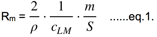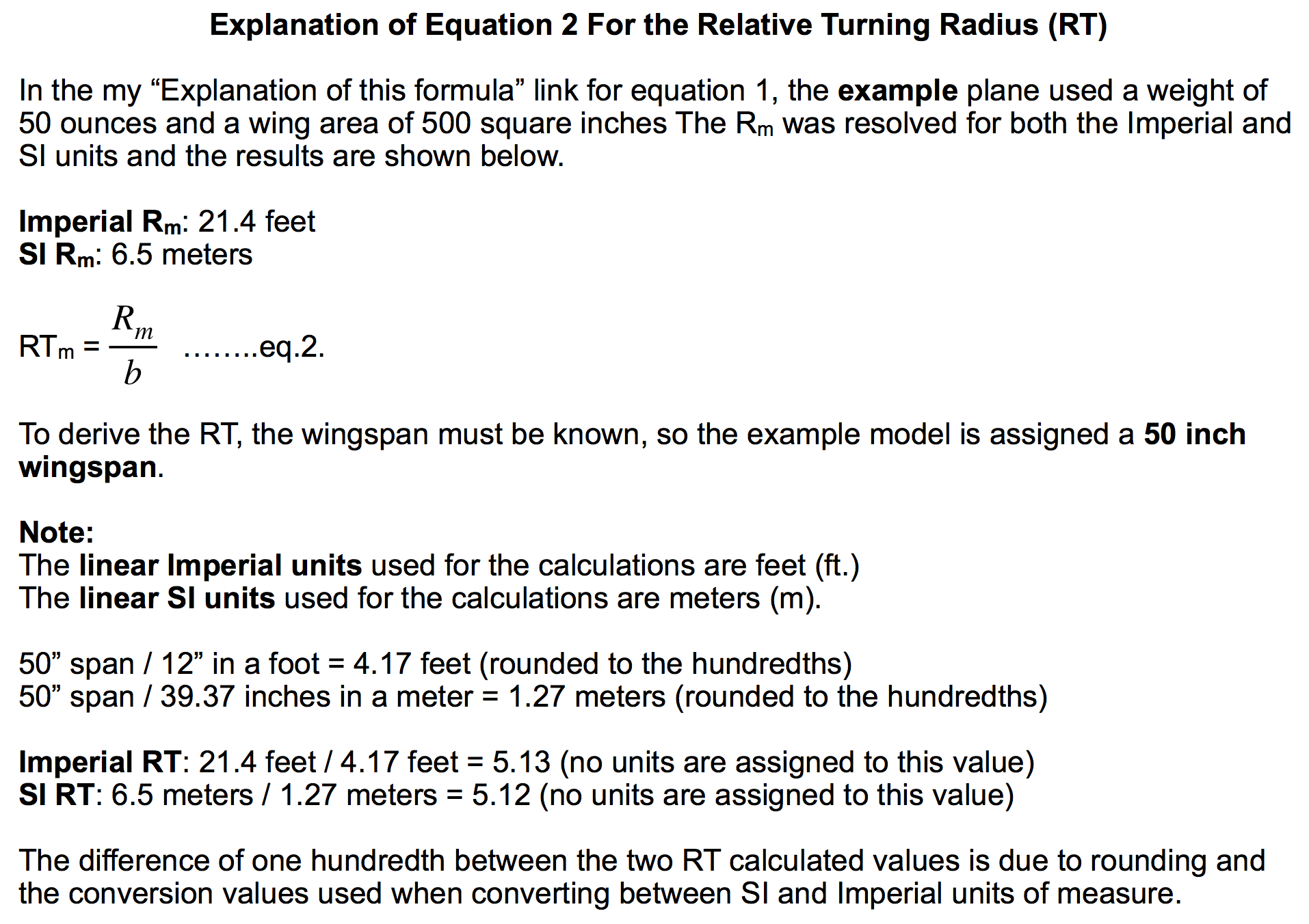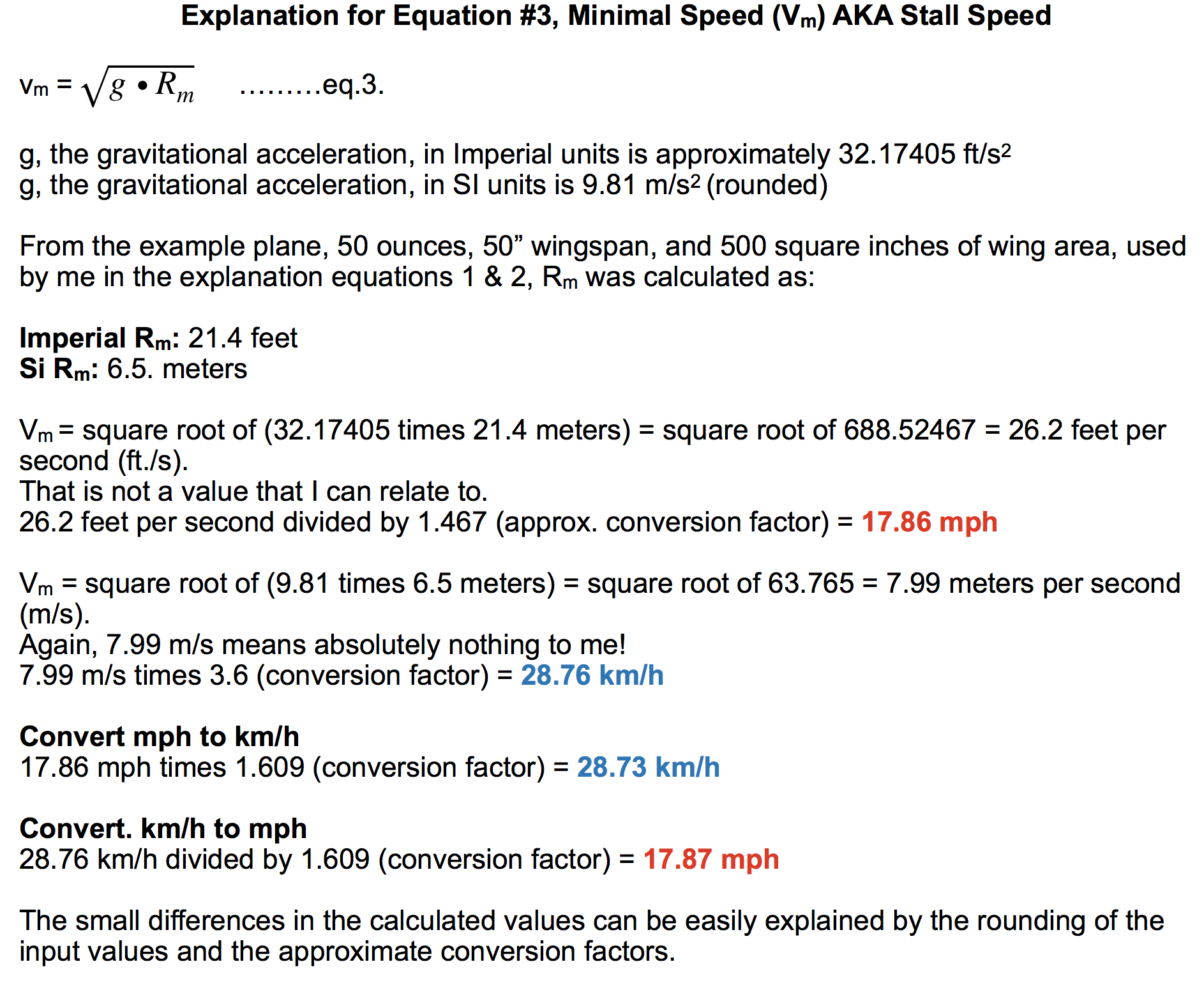1. In turn, the lift force (FL) and the centrifugal force (FC) are equal; by equalizing the eq.L with the eq.C we get R = (2/ρ) * (1/cL) * (m/S). The most interesting is the minimal turning radius (Rm) which we get if the wing's angle of attack is maximal, hence the cL is also maximal (cLM), so: Explanation of this formula      This is the minimal achievable turning radius of the model, measured in the absolute units of length (meters etc). This equation is valid only when the lift force (FL) in turn is much bigger than the weight of model (FG), the condition which is practically fulfilled if a model is turning close to the Rm.      2. The relative turning radius (RT) was introduced in the modeling by the 3D Wing Loading approach and is certainly a reasonable concept in this field. Small models are capable of more tight turns than big ones (or genuine airplanes) so their absolute turning radii (Rm) should be somehow connected and compared to the size of models. This is a kind of visual criterion, where we want that the flying of the differently sized models looks about the same when we are performing turns. Here, the turning capability of the model is not measured by the absolute length units but by the wingspan of model (b), so the minimal relative turning radius (RTm) is defined as: Explanation of this formula      3. The minimal speed (vm) is the third performance parameter we can get from the basic equations. The model maintains level flight at minimal speed if its weight (FG) is equal to the lift force (FL) at the maximal angle of attack (at cLM); by equalizing the eq.L with the eq.G we get the equation for the minimal speed vm = √(2 * g/ρ) * √(1/cLM) * √(m/S). If we use the already calculated Rm (eq.1) and insert it into the equation for the vm we get its much shorter form: Explanation of this formula      We see that all three performance parameters (Rm, RTm and vm) are based, directly or indirectly, on the parameter m/S, used in the 2DWL approach.      These results are, of course, not something new; they can be found, although in different forms, in the literature for aerodynamics for many years. The specific one, and rarely used (if at all), is only the minimal relative turning radius (RT) which will be used later for comparing some performances of models.      In all calculations (examples) herein, the value 1.1 for the maximal lift coefficient (cLM) is used (the mean value between 1.0 and 1.2 for the majority of wing profiles for models without additional high-lift devices). If a model has such devices, they can significantly enlarge the cLM (from approximately 1 to even 2 or more) and the minimal speed (vm) at landing is much lower.      One of the properties is also the wing's aspect ratio (AR = b2/S). At short and wide wings, low AR can lower the value of cLM; this can somewhat affect the calculated performance parameters.      Let's make an example. If a model has the wingspan b =1.3 m, wing area S=0.38 m2, mass m = 2.2 kg and cLM = 1.1, it has the following performance parameters: the minimal turning radius (Rm) is 8.42 m (eq.1), the minimal relative turning radius (RTm) is 6.48 (eq.2) and the minimal speed (vm) is 9.09 m/s (32.7 km/h) (eq.3); its 2D wing loading (m/S) is 5.79 kg/m2 (57.9 g/dm2). The Calculations KM 4.2 Scaling models with the 2DWL      Now we shall use the above three equations at scaling the models. The scaling in our case assumes that the initial (basic) and the scaled model are of the same type which means that their outlines (geometry) are the same. How the changed model is built inside and with what kind of materials is of no importance at this point as this affects only its mass and will be discussed separately a bit later.      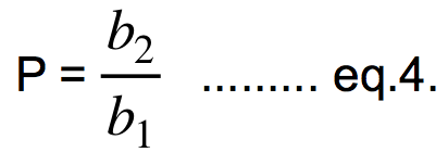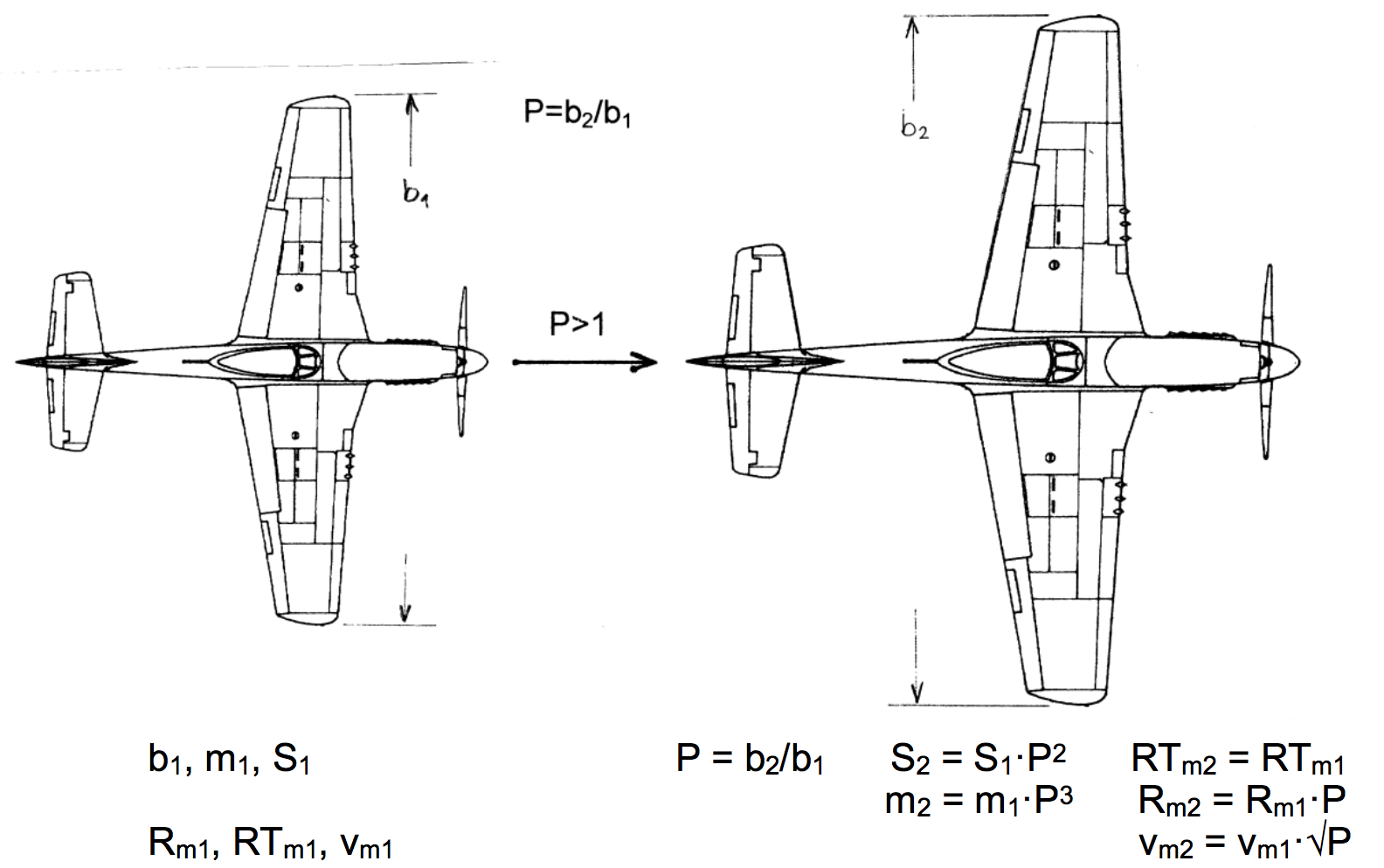By the size of scaling we mean that the wingspan of model is altered, so the wingspan of the basic model b1 will be changed to b2. We define this one dimensional (linear) scaling factor P as:      The P works in both directions; if P>1, model is scaled up (enlarged), if P<1, model is scaled down (reduced) in size.      The chosen condition at scaling, discussed here, is that both models must have the same performance as far as the relative turning radius is concerned, so the RTm2 must be equal to the RTm1. (Reminder: m = mass AKA weight, b = wingspan, and S = wing area KM) Using the eq.1 and the eq.2 we get first m1/(b1 * S1) = m2/(b2 * S2) and then by using the eq.4 we get m2 = m1 * P * (S2/S1). As the areas have two dimensions, they scale by the P2, hence S2 = S1 * P2 so and finally we get: m2 = m1 * P3 ...... eq.5.      We see that the mass of the enlarged (or reduced) model must increase (or decrease) exactly by the scaling factor P on the power of three to achieve the condition mentioned above (RTm2 = RTm1).      Based on the above given relations, the m/S is also scaled:      As the wingspan (b) is scaled by the P and the wing area (S) by the P2, the aspect ratio of the wing does not change at scaling (AR2 = AR1).      Now we shall take a look at how the performance parameters are changed. The chosen condition at our scaling is that the RT stays the same; but the other two performance parameters change. By using the eq.1 and the eq.6 we get: Rm2 = Rm1 * P ......eq.7, and by using the equations 3 and 7 we get: vm2 = vm1 * √P .....eq.8.      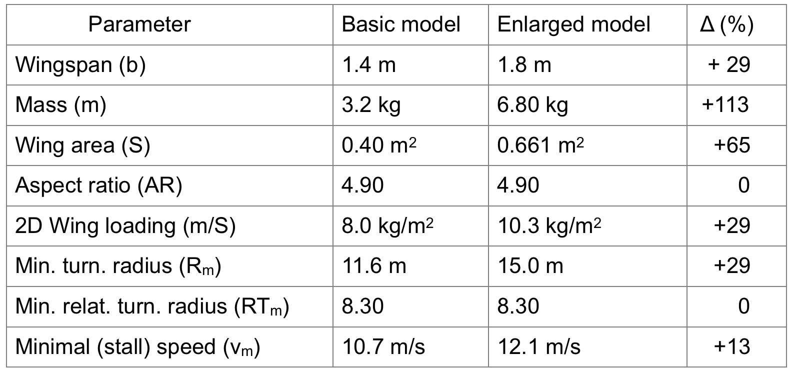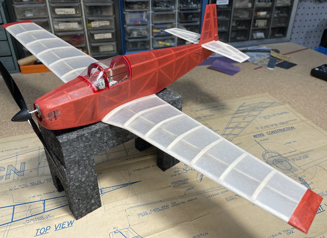As an example we are going to scale a basic model (Mustang) for which we have a proven plan and all necessary data (m1, b1, S1) and enlarge it. Let's take that the basic model has m1 = 3.2 kg, b1 = 1.40 m and S1 = 0.40 m2. Now we choose to enlarge its wingspan to b2 = 1.80 m which means that the scaling factor P is 1.286. The table 1 and the drawing show us what happens with the properties and the performance parameters in this case. Table 1 The Calculations KM      These results give us first, the scaled (target) mass m2 (6.80 kg) of the enlarged model which preserves the model's relative turning radius (RTm) and second, they show us that the Rm and vm are not preserved; they are changed and also scaled differently: Rm by the P and vm by the √P.      Finally we shall shed some light on what can happen with the mass of a model when it is scaled.      As far as building is concerned, there are two possibilities.      The first one is based on the supposition that we have more or less a classically built model (mainly from the wood) and we retain its construction and materials. When the model is for instance scaled up, all three dimensions of building materials increase, their volume increases by the P3 and also their masses by the P3, if the specific mass densities of materials are the same. This is the case presented in the table 1. Some parts (propulsion systems, batteries etc) cannot be scaled continuously and their masses change in jumps. But with some luck, the mass of the built scaled model will be somewhere in the proximity of the calculated target mass (m2) and all results of the scaling are applicable.      The other possibility takes place when the mass of the built model (denoted here by m'2) is not equal to the target mass (m2) calculated from the scaling procedure. If we are determined to build the enlarged model differently than the basic one, and for instance as light as possible, only the outer geometry of the model is preserved, but the inner construction is different, like when we use more modern, lighter and sturdier materials or sacrifice some of its firmness, so the mass of the enlarged model is lower than the calculated target mass. This is a special case of scaling, where the geometry of model is scaled but its mass is not. As the mass is present in all three equations for performance parameters they also change; we get a new, different model with its proper (not scaled) performances, which can be calculated only when we put the finished model (ready to fly) on the scale to obtain its mass (m'2).      Using the Mustang data from the above as an example, let's take it that we have built the enlarged model much lighter and its mass (m'2) is only 5.7 kg instead 6.8 kg (m2). In this case, calculations show that the mass (m), m/S, Rm and RTm are all about 16% lower and the vm is about 8.3% lower. 4.3 Comparing different models with the 2DWL      For this purpose, the 2DWL parameter m/S (wing area loading KM) can be used in two ways. First, for some descriptive and approximate comparison of performances (without the math). As the m/S plays a role in all three performance equations, it tells us that the Rm, RTm and vm are bigger if the m/S is bigger and vice versa; yet this gives us only the information on the direction of change but not on its size.      There also exist some tables (lists, graphs) which loosely link the m/S with the types, purposes and performances of models; roughly speaking gliders would have the m/S somewhere between 20 and 50 g/dm2, average middle sized models from 50 to 100 g/dm2, bigger and heavier models (replicas etc) above 100 g/dm2, not to mention giant models which may have this number even much higher. But this can be misleading; for instance there are bigger and sturdy gliders (for slope flying) with the m/S in the vicinity of 100 g/dm2 and there are also some middle sized and lightly built acrobatic models with the m/S around 50 g/dm2, which are very agile due to their low wing loading.      There are two problems with these kinds of comparisons; the first one is that we usually do not compare directly the performances but the types of models and the second one is the relativity (subjectivity) of the criteria so the results are sometimes pretty close to guesswork.      On the other hand, the 2DWL enables us to get a more exact and objective insight into some of model performances. If we have two different models, all their properties and performance parameters are probably different in any respect. By using the equations 1, 2 and 3 (and also the eq.4 to eq.8) we can get tangible (numerical) results which show us also the size of differences between them.      The performance parameters in the 2DWL approach also enables us to make comparisons at some other kind of conditions.      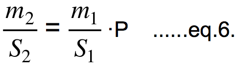For instance, if we want that, for any reason, two models must have the same wing loading (m2/S2 = m1/S1) but have otherwise different properties we see immediately from the equations 1, 2 and 3 that in this case the turning radius (Rm) and the minimal speed (vm) of both models are the same, but the relative turning radii (RTm) are different if the wingspans (b) are different. 5. 3D Wing Loading 5.1 3DWL approach      In the article "3D Wing Loadings", by Larry Renger, two goals are set.      First, if we scale some basic model in size (up or down) and want to retain the performance parameter RTm in the scaled one, the new model must have a certain correct (target) weight and the 3DWL enable us to calculate it; this is the same condition and aim as in the case of 2DWL approach.      The second goal is actually a group of statements which says that we can scale, estimate performances and compare scaled and different models with the 3DWL easily and more accurately than with the 2DWL.      To get the target mass at scaling, several equations are brought forward; for calculations, the 3DWLs article uses only one of them (eq.#4) , which includes (beside the mass) the wingspan and the wing area, and all conclusions are based on it. Another interesting and often used one in practice is the eq.#1, which includes only the wing area and will be discussed separately.      To begin with, we shall take a look at the first goal. 5.2 Scaling models with the 3DWL (Please note that two different methods of deriving the wing cube loading are discussed in the following section. To keep the derived wing cube loadings separate, a bold face lowercase k is used for Larry Lenger's equation #4 and a bold face uppercase K is used for his equation #1. 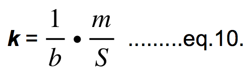KM) 5.2.1 Scaling with the Lenger eq.# 4      To determine the mass of a scaled model under the condition that it retains the relative turning radius (RTm) of the basic one, the 3DWL uses the same or similar equations from the physics and aerodynamics as were used for the calculations in the 2DWL, but combines them in a rather different way, so the result, (the scaled mass) using the 3DWL factor k4 (from now on named the k), given in the eq.#4 in the 3DWLs article, is W = k * S * b. For the reasons mentioned at the beginning of this article, this equation will be written here in the form: m = k * b * S .......eq.9.      For calculating the target mass by the 3DWL approach we need to know the k explicitly so:      First, we must calculate the k for the basic model from the eq.10 (k1 = m1/(b1 * S1)). As the condition here is that both models have the same RTm (hence k2= k1) we get from the eq.9 the target mass of the scaled model: m2 = k1 * b2 * S2 .....eq.11.      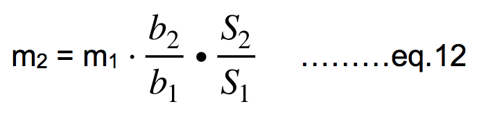The scaled mass can be also directly calculated (in one step) from the eq.12 (see bellow), which is the combination of the eq.10 and the eq.11.      Let's make an example using data from the Mustang scaling case again. By using the eq.10 we get k1= 5.71 kg/m3 and inserting this into the eq.11 we get m2 = 6.80 kg. This is the same number which we have got already from the eq.5 of the 2DWL. This is understandable; if the math and physics from the field of aerodynamics were used correctly in both approaches, that is what we expect.      If we use the condition k2 = k1 and put the eq.10 into it, we get m2/(b2 * S2) = m1/(b1 * S1) and from there:      As b2/b1 is scaling factor P from the 2DWL and as areas are scaled by the P2, hence the wing area S2 is S1 * P2 and the eq.12 can be written as m2 = m1 * P3. We see that the eq.11 in the 3DWL is exactly equivalent to the eq.5 in the 2DWL and either of them can be used equally well at scaling the mass. 5.2.2 Scaling with the Lenger eq.#1      The derivation of the eq.#1 is not given. However, it is pointed out in the Larry Renger's article that the K is also based on aerodynamics (lift force etc.) and not on some mathematical manipulations. Here, the eq.#1 is written as the eq.13. The factor K1 from the eq.#1 is here renamed and the letter K is used instead to avoid possible confusions. So the equation in this case has the shape: m = K * √S3 ... eq.13.      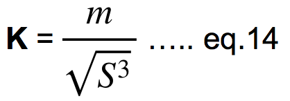As we need the K explicitly, we get it from the eq.13:      At scaling, the procedure to get the scaled mass is the same as was in the case of the k. First, we must calculate the K of the basic model (K1 = m1/√S13) and then put it into the equation for the scaled mass and we get: m2 = K1 * √S23 ... eq.15.      Here also, the scaled mass can be calculated directly if we combine the eq.14. and eq.15 and from there we get: m2 = m1 * √(S2/S1)3 ... eq.16.      The example once more uses the data from the Mustang case (m1 = 3.2 kg, S1 = 0.40 m2 and S2 = 0.661 m2). First, we get K1 = 12.65 kg/m3 and from there m2 = 6.80 kg. Again, the numeric result is the same as was in both previous cases of scaling with the k and with the 2DWL approach (m/S). If we make some calculations we see why. If we put the expression S2 = S1 * P2 into the eq.16 we get m2 = m1 * √P6 and from there m2 = m1 * P3. So the eq.16 is exactly equivalent to the eq.5 in the 2DWL.      We see that for scaling models (retaining the geometry and calculating the target mass at the condition RTm2 = RTm1) we do not need any of the factors derived within the 3DWL (k, K), only some properties of models (m, b and S) are needed and any of the equations 5, 12 or 16 can be used. To put it differently, this aspect of the 3DWL is already comprehended in the 2DWL.      So far so good. 5.3 Comparing different models with the 3DWL      This is the second subject of the 3DWLs article (and also of some others). In this case we compare, by using the factors k (or K) from the 3DWL, a model with some other model (or a group of models), which have generally different all properties m, b, S and also m/S; this is usually the prevailing situation.      The genuine goal at introduction of the 3DWL was, to infer from the history, to get the mass of the scaled model at the condition that it should "fly the same" or "perform the same" as the basic one. The criterion for this is clearly defined in the 3DWLs article: the minimal turning radius of both models must be the same number of wingspan lengths (b) which means that they should have the same relative turning radius (RTm). It appears that only later on, the factors k and K were adopted as a kind of independent and general comparison tools regarding different models.      In the case of the 3DWL factors k and K, tables can also be made which loosely link both factors to the performances of different types and sizes of models, but the problems with them are the same as were already mentioned at the 2DWL tables: the results are sometimes indistinct and can be misleading. The table 2 in the 3DWLs article tells us that a lighter models (for instance soaring gliders) might have the k around 0.7 kg/m3 (0.00041 oz/in3) and heavier R/C scale models around 7 kg/m3 (0,0041 oz/in3) so they will very likely fly quite differently. If we built a new model and calculate its k or K, we can place it somewhere in such table within a group of other models, but this gives us only a limited or even misleading information in some respects about its performances (see bellow).      So here something must be said about two misconceptions which are present in the 3DWL.      The first one is the statement that we can compare models with the K more conveniently because the K is independent of the size of models. The concept of size, as far as calculations are concerned, is usually the wingspan (b) of a model as the most appropriate. But what is even more typical for the perception of the size in general and can be given in some measuring units (m2 etc.) is the area of something, which in our case means the area of the wing (S). So for the eq.14 really can't be said that it does not contain any aspect of the size of model if there is S in it! The statement that there are no size elements in the 3DWL treatment is also not supported by the (more appropriate) factor k where both parameters of the size, the wingspan (b) and the wing area (S) are included in the eq.#4 in the 3DWLs article (the eq.9 in the present article).      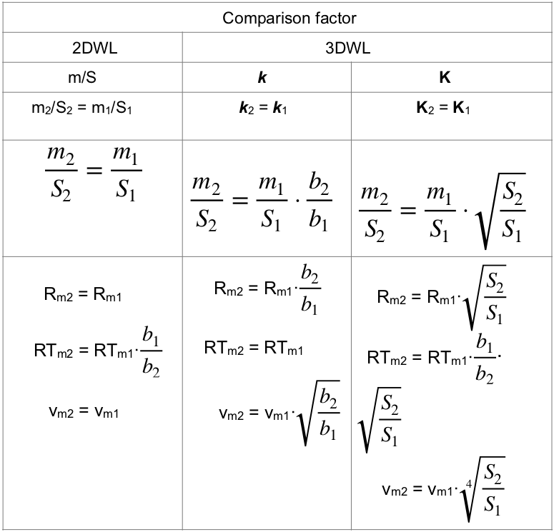The second one is the statement that, if different models have the same numerical value of the k or K, they perform (about) the same; to put it differently, the same value of any of the comparison factors (m/S, k or K) should assure that at least some performance parameters are the same. The equations for general comparison of properties and performances of two different models with all three comparison factors are given in the table 2. The supposition here is that the cLM of both models is the same which eliminates its influence on the Rm. Table 2      We see that if m2/S2 = m1/S1, both models have the same Rm and vm, but their RTm are different. If k2 = k1, both models have the same RTm, but different Rm and vm. If K2 = K1, all performance parameters discussed here (Rm, RTm and vm) between both models are generally different despite the assertions in the 3DWL approach that in this case the models should perform (about) the same because they emerge in the same place (category, level etc.) in some comparison table with the K.      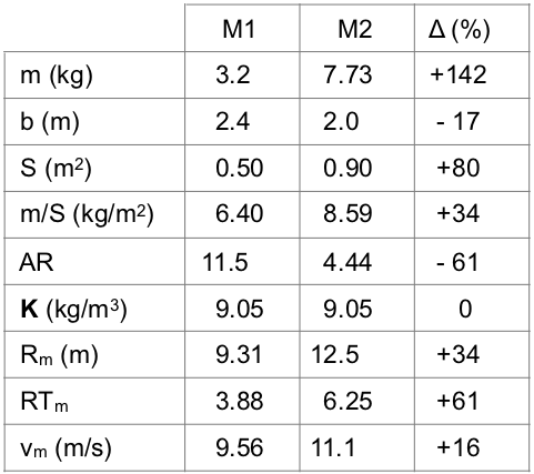Let's make an example where we shall compare two different models (M1 and M2) which have the same K. The data for both models are given in the Table 3. We can freely choose m1, b1, S1, b2 and S2, but m2 must be calculated in such a manner that satisfies the condition K2 = K1 (the equation in the upper right corner in the table 2). The first three rows contain the basic properties of both models, in the next three are some additional calculated properties and in the last three are the performance parameters which we are dealing with in this article. The first model (M1) is close to some middle sized electric powered glider and the second one (M2) is close to some larger classically powered sport or scale type. Table 3      The results show us that despite the fact, that both models have exactly the same value of the K (9.05 kg/m3), their performances Rm, RTm and vm are quite different. And what is even more important, because of the different nature and purpose of these two models (glider, sport type) we also can't expect that some other performance parameters, which depend on many other properties of both models (and which can also be very different) will be the same. So the same value of the K generally does not give us any assurance that models will have the same or similar flying characteristics as far as their objective performance parameters are concerned.      The K is frequently used as a criterion for estimation of flying property named the flyability of models. The flyability is actually not well defined so the connection to the K is pretty loose and arbitrary. However, the m/S and the K do not exclude each other, but are different yardsticks and cover different aspect of flying characteristics; the first one covers objective performance parameters (not only those mentioned here) and the second one some more elusive (hard to calculate and predict in advance) performances. Estimations of different aspects of flyability can be often found in some more thorough reviews of models. 6. Summary      1. All three comparison factors (m/S, k and K) are not some performance parameters but are only a combinations of model properties (m, b, S); with regard to the numerical value of a certain combination, models and their performances can be either loosely grouped (comparison tables) or calculated (equations) or both.      2. All three factors (m/S, k and K) can be used for some descriptive (non-numerical) and approximate comparisons of model performances. This demands some comprehensive assessments, performed by greater number of experienced modelers with greater number of different models to get some more credible comparison tables, which links any of those three factors with different models. In any case, each table is usable only within its own frame of reference (the calculated k can't be used in some table based on the K). Several comparison tables can be found around; some are sketchy, others are quite comprehensive and detailed, but first, they are not always compatible with each other and second, as the results from the above show us, models with the same K generally do not have the same performance parameters. The problem arises because the K is "borrowed" from the scaling procedure (calculation of the scaled mass) and is then used for comparison of performances of different models, which is something else. Also, the comparison factors in the tables (m/S, k or K) are usually not linked to some more tangible performances but to the types, sizes and flyability of models.      3. To compare the abilities of those three factors when we want to use them at calculations of some model performances for quantitative, numerical comparisons, the situation is the following: - the k (eq.10) and the K (eq.14) can not be used directly for any further calculations of performance parameters; there are no equations within the 3DWL approach (in both cases, at the k and the K), which could enable us to calculate any performance parameters with them, because the k and the K are only some middle steps when the target mass is calculated at scaling. Nevertheless, both can be used indirectly. With the help of the eq.10, the k can be transformed into the m/S (m/S = k * b) and from the eq.13, the K can be also transformed into the m/S (m/S = K * √S); these m/S can be than used for calculations of some performances within the frame of the 2DWL. - the most employable is the 2DWL factor m/S. It can be used for some descriptive comparisons, but it enables us also to directly calculate some objective performance parameters such as the absolute minimal turning radius (Rm) and the stall speed (vm) and also some others performances which are usually not very important regarding models but are significant for genuine aircrafts.      So in some statements in the 3DWL's article, unfounded or overstretched capabilities are attributed to the k (and indirectly to the K), which are questionable and also incorrect, such as: - the same model in two different sizes, which have the same k perform (about) the same? This is the case of scaling; we have seen, that only one performance parameter (RTm) is preserved, the others (at least Rm and vm) are changed; - the accuracy of comparison at scaling (by the 3DWL) is way better than by the 2DWL? If we want that both models have the same RTm, the calculated scaled mass is the same in all three approaches; - the k is much more constant than the m/S? If the built scaled model has the mass which corresponds to the eq.11 (the target scaled mass), the k of both models is of course the same, but the m/S cannot be the same because at scaling the wingspan (b) is changed (eq.10: m/S = k * b) - the k allows valid comparisons between very different model designs and sizes? If we neglect the possible differences between cLM, this is even more true for the m/S (see Table 2); if the m/S of two different models is the same, we know that two of their performance parameters (Rm and vm) are the same; in the case of the equality of the k, only one is the same (RTm), not to mention the K where none of the performance parameters is the same; - the 2DWL is inadequate theory and is valid for comparison of models in very narrow size and design range? Just the opposite; the 2DWL, based on the m/S, allows us to validate any size and design of models (and genuine aircrafts for that matter) and gives us more information about their performances than the 3DWL comparison factors; - the m/S has limited use? If one cast an eye at literature for aerodynamics this is certainly not the case.      Raising the k (and particularly the K) into the most appropriate and comprehensive comparison tool for model performances and neglecting the m/S (especially in the case of different models but also at scaling) is somehow unusual (to put it mildly). The cherry on the cake is the statement in an article which says that "the wing loading (m/S) is a lousy way to compare models with each other"! 7. Conclusion      Here we were occupying ourselves with only a few performance parameters of models, but there are of course many others (maximal speed, acceleration/deceleration, roll rate, spin characteristics, stability etc); we can also add flying outside the usual flying envelope, for instance well above the critical angle of attack, hovering and so on. All that together with the flying skills of modelers enable us to make an impression on our audience or to please ourselves at flying.      Markets today are flooded with not so expensive models of different kinds, sizes, weights and propulsion systems. If somebody wants to have a new model of a certain size and design, he will most likely buy it. Scaling existing models (and building them from scratch) is less common but is still practiced by more ambitious, enthusiastic and skilled modelers. In both cases a proper tool for comparing performances is sometimes needed; any comparison tool can be used but we must be aware of its deficiencies and limitations to get the correct and useful information about flying properties of our models. References: - Model design & technical stuff by Francis Reynolds, Model Builder (Sept. 1989) - 3D Wing Loadings by Larry Renger, Model Airplane News (Dec. 1997) - Wing Cube Loading by Ken Myers, Ampeer (June 2018) - Aircraft Performance and Design by John D. Anderson, Jr., McGraw-Hill (1999) © by Andrej Marinsek Return to "What's In This Issue" The February EFO Zoom Meeting      The Wednesday, February 9, EFO meeting was held via Zoom.      For unknown reasons, it was a challenge for us to log on, but we finally had seven members in attendance. Photo from Denny Sumner's RC Groups build thread      Denny Sumner, Keith Shaw and Dave Stacer had flown at the Legacy Center that afternoon and Denny had flown his Ace Whitman 18" Mooney Mite (UMX).      There was a lot of discussion about batteries and some "guessing" at how Lithium AA batteries could be rechargeable. 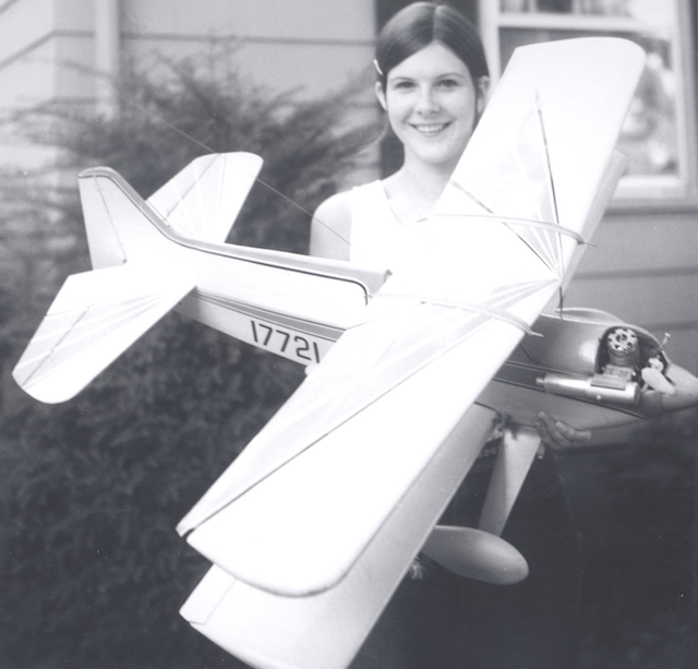Link to these batteries on Amazon      Keith Shaw mentioned that he'd like to do an electric powered version of the original Dreamer biplane. The photo is from Flying Models "store". 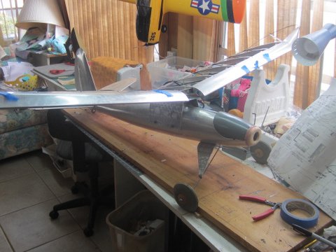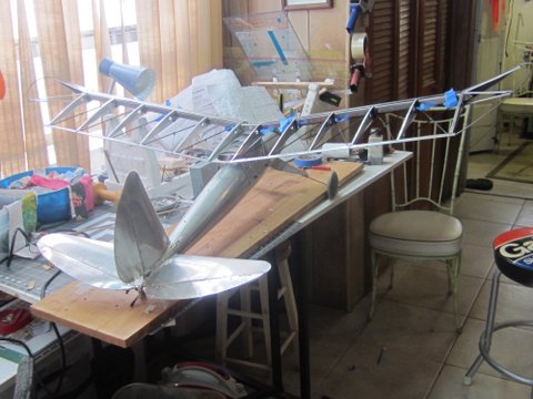Return to "What's In This Issue" Pete Waters' Latest Model From Pete Waters via email      Getting there, 1945 kit I had to have! 4 1/4 lb. all up with a 60 inch span.      It is all aluminum and uses 1/16" squeeze rivets and #2 small screws. Return to "What's In This Issue" Skymasters Indoor Flying starting October 20 through April 13, 2022 From Pete Foss, Skymasters' President via email HELLO INDOOR FLIERS!      We're back for Indoor Flying starting October 20th! I'm very happy to announce that through the efforts of Fred Engleman and Paul Goelz we have an agreement with Reimagine Recreation to fly on Wednesdays at United Wholesale Mortgage Sports Complex (formerly Ultimate Soccer). It was a bit of a struggle dealing with the new owners of the facility and I would really like to thank Fred and Paul for stepping up and pushing us to the finish line!      There are some differences beyond the fact that we will be flying on field 4 (the one in the back) since field 3, where we used to fly, is now a basketball and volleyball arena. Everyone who enters the building for any reason during our time slot MUST SIGN A LIABILITY WAIVER. It would be helpful if you print a copy, sign and bring to your first flying session but we will have printed waivers on hand too. Park out back by field 4. You will not be allowed to enter the front door.      To simplify this year, we went with only Gold (season pass) cards for $150 and single sessions at $10 each. Also, since ReImagine charges Skymasters for each and every pilot who flies, youths and spouses are no longer free.      Here is a direct link to register and purchase a Gold Card or print out a registration form for your first single session.      Hope to see many of you on the 20th, or before, at the Night Fly and Free Tailgate Swap at Skymasters' Field. Indoor Flying - Wednesday, October 20, 2021 - UWM Sports Complex, 837 South Blvd, Pontiac, MI Time: 10:00 Sponsor: Skymasters Indoor Flying At UWM Sports Complex On Field #4 (Park and Enter on the north "back" end of the complex - Wednesdays starting October 20, 2021 thru April 13, 2022 View Event PDF Flyer View Event Map Contact: Fred Engleman Phone: (248) 770-3239 Email: indoorfly@skymasters.org Updated Information 11/01/21: FYI - For those of you who want to park a little closer, we found out that the early morning Wednesday, UWM Training Sessions let out at 10 and the parking lot empties out quickly making more room for us closer to entrance of Field #4. Season Passes are still available online for $150 at www.Skymasters.org. If you have any problems with the online registration process, give me a call at (248) 770-3239. Or you can purchase a $10 Single Session at the door (NOTE: there is no longer an ATM machine in the building, so you will need to bring the proper change/cash only). Pilots/Drivers and Spectators you can read the Indoor Flying Rules, Schedule and Release Form Liability Form on-line at www.Skymasters.org Each Pilot/Driver and Spectator will be required to sign a onetime Release Form Liability Form. 11/10/21: It seemed to work well that pilots who arrived few minutes after 10 were able to park closer to entrance for Field #4. With a ceiling height of 75 feet pilots do not have luxury of flying 3 mistakes high. We are also surrounded by 4 walls, fellow pilots and spectators all around. The utmost care must be taken when flying at all times. Pilots flying the faster delta wing planes must give way to slower planes. That said, if you are flying a slower plane, you may want to land when faster planes are in the air. Batteries only last a short time and you can return to the air to fly without costly mishaps. Everyone wants to have a good time and return home with our planes intact. A quick reminder, if you are charging batteries the batteries must be in or on a fire retardant surface like a lipo sack. No charged or discharged batteries may be left at UWMSC. Return to "What's In This Issue" Indoor Flying at the Legacy Center in Brighton, MI      Indoor flying takes place from November 3rd, 2021 until March 30th, 2022 at the Legacy Center Sports Complex, 9299 Goble Dr., Brighton, MI 48116, phone: 810.231.9288, on Wednesdays from 12:30 PM until 2:30 PM.      The cost is $10 per drop-in session. Return to "What's In This Issue" To Reach Ken Myers, you can land mail to the address at the top of the page. My E-mail address is: KMyersEFO@theampeer.org EFO WEB Site